Opening and Writing SWxSOC Affiliated Data¶

Overview¶

The SWXData class provides a convenient and efficient way to work with SWxSOC affiliated mission science CDF data files. The point of this class is to simplify data management, enhance data discovery, and facilitate adherence to CDF standards.

CDF (Common Data Format) files are a binary file format commonly used by NASA scientific research to store and exchange data. They provide a flexible structure for organizing and representing multidimensional datasets along with associated metadata. CDF files are widely used in space physics. Because of their versatility, CDF files can be complex. CDF standards exist to make it easier to work with these files. International Solar-Terrestrial Physics (ISTP) compliance is a set of standards defined by the Space Physics Data Facility (SPDF). ISTP compliance ensures that the data adheres to specific formatting requirements, quality control measures, and documentation standards. Uploading CDF files to the NASA SPDF archive requires conforming to the ISTP guidelines.

The CDF C library must be properly installed in order to use this package to save and load CDF files. The CDF library can be downloaded from the SPDF CDF Page to use the CDF libraries in your local environment. Alternatively, the CDF library is installed and available through the development Docker container environment. For more information on the Docker container please see our Development Environment Page.

To make it easier to work with SWxSOC affiliated mission data, the SWXData class facilitates the abstraction of CDF files. It allows users to read and write instrument data and is compliant with PyHC expectations. Data is stored in a combination of TimeSeries, NDData, and NDCollection objects. Metadata is stored in dictionaries, with a dataset level dict for global metadata, and variable-level dict`s for variable attributes. By loading the contents of a CDF file into these data structures, it becomes easier to manipulate, analyze, and visualize the data. Additionally, metadata attributes associated with the table allow for enhanced documentation and data discovery. The :py:class:`~swxsoc.swxdata.SWXData class aims to provide a simplified interface to reading and writing data and metadata to CDF files while automatically handling the complexities of the underlying CDF file format.

Creating a `SWXData` object¶

Creating a SWXData data container from scratch involves four pieces of data:

timeseries (required) - an TimeSeries or
dict[str : ~astropy.timeseries.TimeSeries] containing one or more time variables, and any other time-varying scalar measurements. Time-varying measurements should appear in the table as columns with their associates time variable as the first column.
support (optional) - a dict[astropy.nddata.NDdata | astropy.units.Quantity] containing one
or more non-time-varying (time invariant) measurements, time-invariant support or metadata variables.
spectra (optional) - an NDCollection containing one or more NDCube objects
representing higher-dimensional measurements and spectral data. This data must should be used for all vector or tensor-based measurement data.
meta (optional) - a dict containing global metadata information about the CDF. This data
structure must be used for all global metadata required for ISTP compliance.

Alternatively, a SWXData data container can be loaded from an existing CDF file using the load() function.

Creating `TimeSeries` for `SWXData` `timeseries`¶

A SWXData must be initialized by providing one or more TimeSeries object with at least one measurement. There are many ways to initialize one but here is one example:

>>> import numpy as np
>>> import astropy.units as u
>>> from astropy.timeseries import TimeSeries
>>> example_ts = TimeSeries(
...     time_start='2016-03-22T12:30:31',
...     time_delta=3 * u.s,
...     data={'Bx': u.Quantity(
...         value=[1, 2, 3, 4],
...         unit='nanoTesla',
...         dtype=np.uint16
...     )}
... )

Be mindful to set the right number of bits per measurement, in this case 16 bits. If you do not, it will likely default to float64 and if you write a CDF file, it will be larger than expected or needed. The valid dtype choices are uint8, uint16, uint32, uint64, int8, int16, int32, int64, float16, float32, float64, float164. You can also create your time array directly

>>> from astropy.time import Time, TimeDelta
>>> import astropy.units as u
>>> from astropy.timeseries import TimeSeries
>>> times = Time('2010-01-01 00:00:00', scale='utc') + TimeDelta(np.arange(100) * u.s)
>>> ts_2 = TimeSeries(
...     time=times,
...     data={'diff_e_flux': u.Quantity(
...         value=np.arange(100) * 1e-3,
...         unit='1/(cm**2 * s * eV * steradian)',
...         dtype=np.float32
...     )}
... )

Note the use of time and astropy.units which provide several advantages over using arrays of numbers and are required by SWXData.

For collections that have multiple Epochs, you can create a dictionary of TimeSeries objects.

>>> from astropy.time import Time, TimeDelta
>>> import astropy.units as u
>>> from astropy.timeseries import TimeSeries
>>> import numpy as np
>>> # Collected at one-second cadence
>>> primary_epoch = Time('2010-01-01 00:00:00', scale='utc') + TimeDelta(np.arange(100) * u.s)
>>> # Collected at 10-second cadence
>>> secondary_epoch = Time('2010-01-01 00:00:00', scale='utc') + TimeDelta(np.arange(10) * (10*u.s))
>>> ts_3 = {
...     'Epoch': TimeSeries(
...         time=primary_epoch,
...         data={'diff_e_flux': u.Quantity(
...             value=np.arange(100) * 1e-3,
...             unit='1/(cm**2 * s * eV * steradian)',
...             dtype=np.float32
...         )}
...     ),
...     'Epoch_state': TimeSeries(
...         time=secondary_epoch,
...         data={'counts': u.Quantity(
...             value=np.arange(10),
...             unit='Celsius',
...             dtype=np.float32
...         )}
...     )
... }

This allows you to have multiple time series in one SWXData object.

Creating a `NDCollection` for `SWXData` `spectra`¶

The SWXData object leverages API functionality of the ndcube package to enable easier analysis of higher-dimensional and spectral data measurements. The main advantage that this package provides in in it’s handling of coordinate transformations and slicing in real-world-coordinates compared to using index-based slicing for higher-dimensional data. For more information about the ndcube package and its API functionality please read the SunPy NDCube documentation.

You can create a NDCollection object using an approach similar to the following example:

>>> import numpy as np
>>> from astropy.wcs import WCS
>>> from ndcube import NDCube, NDCollection
>>> example_spectra = NDCollection(
...     [
...         (
...             "example_spectra",
...             NDCube(
...                 data=np.random.random(size=(4, 10)),
...                 wcs=WCS(naxis=2),
...                 meta={"CATDESC": "Example Spectra Variable"},
...                 unit="eV",
...             ),
...         )
...     ]
... )

The NDCollection is created using a list of tuple containing named (str, NDCube) pairs. Each NDCube contains the required data array, a WCS object responsible for the coordinate transformations, optional metadata attributes as a dict, and an units unit that is used to treat the data array as an Quantity.

Creating a `dict` for `SWXData` `support`¶

The SWXData object also accepts additional arbitrary data arrays, so-called non-record-varying (NRV) data, which is frequently support data. These data are required to be a dict of NDData or Quantity objects which are data containers for physical data. The SWXData class supports both Quantity and NDData objects since one may have advantages for the type of data being represented: Quantity objects in this support dict may be more advantageous for scalar or 1D-vector data while NDData objects in this support dict may be more advantageous for higher-dimensional vector data. A guide to the nddata package is available in the astropy documentation.

>>> from astropy.nddata import NDData
>>> const_param = u.Quantity(value=[1e-3], unit="keV", dtype=np.uint16)
>>> const_param.meta = {"CATDESC": "Constant Parameter", "VAR_TYPE": "support_data"}
>>> data_mask = NDData(data=np.eye(100, 100, dtype=np.uint16))
>>> data_mask.meta = {"CATDESC": "Data Mask", "VAR_TYPE": "support_data"}
>>> example_support_data = {
...     "const_param": const_param,
...     "data_mask": data_mask
... }

Metadata passed in through the NDData object is used by SWXData as variable metadata attributes required for ISTP compliance.

Creating a `dict` for `SWXData` `meta`¶

You must create a dict or OrderedDict containing the required CDF global metadata. The class function global_attribute_template() will provide you an empty version that you can fill in. Here is an example with filled in values.

>>> input_attrs = {
...     "DOI": "https://doi.org/<PREFIX>/<SUFFIX>",
...     "Data_level": "L1>Level 1",  # NOT AN ISTP ATTR
...     "Data_version": "0.0.1",
...     "Descriptor": "EEA>Electron Electrostatic Analyzer",
...     "Data_product_descriptor": "odpd",
...     "HTTP_LINK": [
...         "https://spdf.gsfc.nasa.gov/istp_guide/istp_guide.html",
...         "https://spdf.gsfc.nasa.gov/istp_guide/gattributes.html",
...         "https://spdf.gsfc.nasa.gov/istp_guide/vattributes.html"
...     ],
...     "Instrument_mode": "default",  # NOT AN ISTP ATTR
...     "Instrument_type": "Electric Fields (space)",
...     "LINK_TEXT": [
...         "ISTP Guide",
...         "Global Attrs",
...         "Variable Attrs"
...     ],
...     "LINK_TITLE": [
...         "ISTP Guide",
...         "Global Attrs",
...         "Variable Attrs"
...     ],
...     "MODS": [
...         "v0.0.0 - Original version.",
...         "v1.0.0 - Include trajectory vectors and optics state.",
...         "v1.1.0 - Update metadata: counts -> flux.",
...         "v1.2.0 - Added flux error.",
...         "v1.3.0 - Trajectory vector errors are now deltas."
...     ],
...     "PI_affiliation": "HERMES",
...     "PI_name": "HERMES SOC",
...     "TEXT": "Valid Test Case",
... }

Here is an example using the global_attribute_template() function to create a minimal subset of global metadata attributes:

>>> from swxsoc.swxdata import SWXData
>>> input_attrs = SWXData.global_attribute_template("eea", "l1", "1.0.0")

Using Defined Elements to create a `SWXData` Data Container¶

Putting it all together here is instantiation of a SWXData object:

>>> from swxsoc.swxdata import SWXData
>>> example_sw_data = SWXData(
...     timeseries=example_ts,
...     support=example_support_data,
...     spectra=example_spectra,
...     meta=input_attrs
... )

For a complete example with instantiation of all objects in one code example:

>>> import numpy as np
>>> from astropy.time import Time, TimeDelta
>>> import astropy.units as u
>>> from astropy.timeseries import TimeSeries
>>> from ndcube import NDCube, NDCollection
>>> from astropy.nddata import NDData
>>> from swxsoc.swxdata import SWXData
>>> # Collected at one-second cadence
>>> primary_epoch = Time('2010-01-01 00:00:00', scale='utc') + TimeDelta(np.arange(100) * u.s)
>>> # Collected at 10-second cadence
>>> secondary_epoch = Time('2010-01-01 00:00:00', scale='utc') + TimeDelta(np.arange(10) * (10*u.s))
>>> # Create a TimeSeries structure
>>> ts = {
...     'Epoch': TimeSeries(
...         time=primary_epoch,
...         data={'diff_e_flux': u.Quantity(
...             value=np.arange(100) * 1e-3,
...             unit='1/(cm**2 * s * eV * steradian)',
...             dtype=np.float32
...         )}
...     ),
...     'Epoch_state': TimeSeries(
...         time=secondary_epoch,
...         data={'counts': u.Quantity(
...             value=np.arange(10),
...             unit='Celsius',
...             dtype=np.float32
...         )}
...     )
... }
>>> # Create a Support Structure
>>> support_data = {
...     "data_mask": NDData(
...         data=np.eye(10, 10, dtype=np.uint16),
...         meta={"CATDESC": "Data Mask", "VAR_TYPE": "support_data"}
...     ),
... }
>>> # Create a Spectra structure
>>> spectra = NDCollection(
...     [
...         (
...             "example_spectra",
...             NDCube(
...                 data=np.random.random(size=(10, 10)),
...                 wcs=WCS(naxis=2),
...                 meta={"CATDESC": "Example Spectra Variable"},
...                 unit="eV",
...             ),
...         )
...     ]
... )
>>> # Create a Support Structure
>>> support_data = {
...     "data_mask": NDData(data=np.eye(100, 100, dtype=np.uint16))
... }
>>> # Create Global Metadata Attributes
>>> input_attrs = SWXData.global_attribute_template("eea", "l1", "1.0.0")
>>> # Create SWXData Object
>>> sw_data = SWXData(
...     timeseries=ts,
...     support=support_data,
...     spectra=spectra,
...     meta=input_attrs
... )

The SWXData is mutable so you can edit it, add another measurement column or edit the metadata after the fact. Your variable metadata can be found by querying the measurement column directly.

>>> example_sw_data.timeseries['Bx'].meta.update(
...     {"CATDESC": "X component of the Magnetic field measured by HERMES"}
... )
>>> example_sw_data.timeseries['Bx'].meta 

For multiple epoch variables, you have to addess measurements through the timeseries dictionary, keyed by the epoch name:

>>> sw_data.timeseries['Epoch']['diff_e_flux'].meta.update(
...     {"CATDESC": "Differential Electron Flux measured by HERMES"}
... )
>>> sw_data.timeseries['Epoch']['diff_e_flux'].meta 

The class does its best to fill in metadata fields if it can and leaves others blank that it cannot. Those should be filled in manually. Be careful when editing metadata that was automatically generated as you might make the resulting CDF file non-compliant.

Creating a `SWXData` from an existing CDF File¶

Given a current CDF File you can load it into a SWXData by providing a Path to the CDF file:

>>> from pathlib import Path
>>> from swxsoc.swxdata import SWXData
>>> data_path = Path("hermes_eea_default_ql_20240406T120621_v0.0.1.cdf")
>>> sw_data = SWXData.load(data_path) 

The SWXData can the be updated, measurements added, metadata added, and written to a new CDF file.

Adding data to a `SWXData` Container¶

A new set of measurements or support data can be added to an existing instance. Remember that new measurements must have the same time stamps as the existing ones and therefore the same number of entries. Support data can be added as needed. You can add the new measurements in one of two ways.

The more explicit approach is to use add_measurement() function:

>>> data = u.Quantity(np.arange(len(example_sw_data.timeseries['Bx'])), 'Gauss', dtype=np.uint16)
>>> example_sw_data.add_measurement(
...     measure_name="By",
...     data=data,
...     meta={"CATDESC": "Y component of the Magnetic field measured by HERMES"}
... )

To add non-time-varying support data use the add_support() function:

>>> sw_data.add_support(
...     name="Calibration_const",
...     data=u.Quantity(value=[1e-1], unit="keV", dtype=np.uint16),
...     meta={"CATDESC": "Calibration Factor", "VAR_TYPE": "support_data"},
... )
>>> sw_data.add_support(
...     name="Data Mask",
...     data=NDData(data=np.eye(5, 5, dtype=np.uint16)),
...     meta={"CATDESC": "Diagonal Data Mask", "VAR_TYPE": "support_data"},
... )

Adding metadata attributes¶

Additional CDF file global metadata and variable metadata can be easily added to a SWXData data container. For more information about the required metadata attributes please see the CDF Format Guide

Global Metadata Attributes¶

Global metadata attributes can be updated for a SWXData object using the object’s meta parameter which is an OrderedDict containing all attributes.

Required Global Attributes¶

The SWXData class requires several global metadata attributes to be provided upon instantiation:

Descriptor
Data_level
Data_version

A SWXData container cannot be created without supplying at lest this subset of global metadata attributes. For assistance in defining required global attributes, please see the global_attribute_template() function.

Derived Global Attributes¶

The SWXSchema class derives several global metadata attributes required for ISTP compliance. The following global attributes are derived:

CDF_Lib_version
Data_type
Generation_date
swxsoc_version
Logical_file_id
Logical_source
Logical_source_description

For more information about each of these attributes please see the CDF Format Guide

Using a Template for Global Metadata Attributes¶

A template of the required metadata can be obtained using the global_attribute_template() function:

>>> from collections import OrderedDict
>>> from swxsoc.swxdata import SWXData
>>> SWXData.global_attribute_template()
OrderedDict([('Data_level', None),
         ('Data_version', None),
         ('Descriptor', None),
         ('Discipline', None),
         ('Instrument_type', None),
         ('Mission_group', None),
         ('PI_affiliation', None),
         ('PI_name', None),
         ('Project', None),
         ('Source_name', None),
         ('TEXT', None)])

You can also pass arguments into the function to get a partially populated template:

>>> from collections import OrderedDict
>>> from swxsoc.swxdata import SWXData
>>> SWXData.global_attribute_template(
...     instr_name='eea',
...     data_level='l1',
...     version='0.1.0'
... )
OrderedDict([('Data_level', 'L1>Level 1'),
         ('Data_version', '0.1.0'),
         ('Descriptor', 'EEA>Electron Electrostatic Analyzer'),
         ('Discipline', None),
         ('Instrument_type', None),
         ('Mission_group', None),
         ('PI_affiliation', None),
         ('PI_name', None),
         ('Project', None),
         ('Source_name', None),
         ('TEXT', None)])

This can make the definition of global metadata easier since instrument teams or users only need to supply pieces of metadata that are in this template. Additional metadata items can be added if desired. Once the template is instantiated and all attributes have been filled out, you can use this during instantiation of your SWXData container.

Variable Metadata Attributes¶

Variable metadata requirements can be updated for a SWXData variable using the variable’s meta property which is an OrderedDict of all attributes.

Required Variable Attributes¶

The SWXData class requires one variable metadata attribute to be provided upon instantiation:

CATDESC : (Catalogue Description) This is a human readable description of the data variable.

Derived Variable Attributes¶

The SWXSchema class derives several variable metadata attributes required for ISTP compliance.

DEPEND_0
DISPLAY_TYPE
FIELDNAM
FILLVAL
FORMAT
LABLAXIS
SI_CONVERSION
UNITS
VALIDMIN
VALIDMAX
VAR_TYPE

For more information about each of these attributes please see the CDF Format Guide

Using a Template for Variable Metadata Attributes¶

A template of the required metadata can be obtained using the measurement_attribute_template() function:

>>> from collections import OrderedDict
>>> from swxsoc.swxdata import SWXData
>>> SWXData.measurement_attribute_template()
OrderedDict([('CATDESC', None)])

If you use the add_measurement() function, it will automatically fill most of them in for you. Additional pieces of metadata can be added if desired.

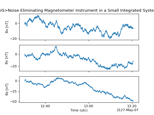
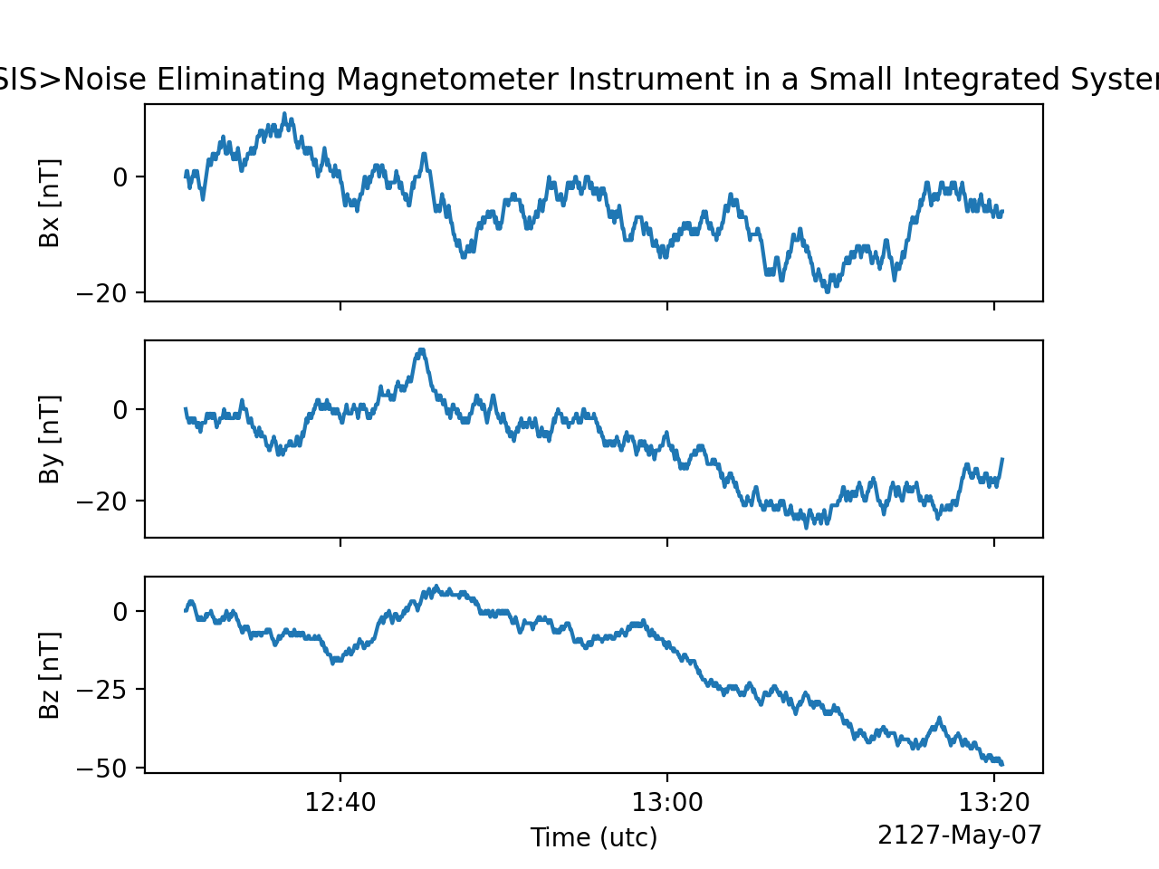
Visualizing data in a `SWXData` Container¶

The SWXData provides a quick way to visualize its data through plot. By default, a plot will be generated with each measurement in its own plot panel.

>>> import numpy as np
>>> import matplotlib.pyplot as plt
>>> import astropy.units as u
>>> from astropy.timeseries import TimeSeries
>>> from swxsoc.swxdata import SWXData
>>> bx = np.concatenate([[0], np.random.choice(a=[-1, 0, 1], size=1000)]).cumsum(0)
>>> by = np.concatenate([[0], np.random.choice(a=[-1, 0, 1], size=1000)]).cumsum(0)
>>> bz = np.concatenate([[0], np.random.choice(a=[-1, 0, 1], size=1000)]).cumsum(0)
>>> ts = TimeSeries(time_start="2016-03-22T12:30:31", time_delta=3 * u.s, data={"Bx": u.Quantity(bx, "nanoTesla", dtype=np.int16)})
>>> input_attrs = SWXData.global_attribute_template("nemisis", "l1", "1.0.0")
>>> sw_data = SWXData(timeseries=ts, meta=input_attrs)
>>> sw_data.add_measurement(measure_name=f"By", data=u.Quantity(by, 'nanoTesla', dtype=np.int16))
>>> sw_data.add_measurement(measure_name=f"Bz", data=u.Quantity(bz, 'nanoTesla', dtype=np.int16))
>>> fig = plt.figure()
>>> sw_data.plot() 
>>> plt.show() 

(Source code, png, hires.png, pdf)

Writing a CDF File¶

The SWXData class writes CDF files using the pycdf module. This can be done using the save() method which only requires a Path to the folder where the CDF file should be saved. If no path is provided it writes the file to the current directory. This function returns the full Path to the CDF file that was generated. From this you can validate and distribute your CDF file.

Validating a CDF File¶

The SWXData uses the istp module for CDF validation, in addition to custom tests for additional metadata. A CDF file can be validated using the validate() method and by passing, as a parameter, the full Path to the CDF file to be validated:

>>> from swxsoc.util.validation import validate
>>> validation_errors = validate(cdf_file_path) 

This returns a list[str] that contains any validation errors that were encountered when examining the CDF file. If no validation errors were found the method will return an empty list.

Opening and Writing SWxSOC Affiliated Data¶

Overview¶

Creating a `SWXData` object¶

Creating `TimeSeries` for `SWXData` `timeseries`¶

Creating a `NDCollection` for `SWXData` `spectra`¶

Creating a `dict` for `SWXData` `support`¶

Creating a `dict` for `SWXData` `meta`¶

Using Defined Elements to create a `SWXData` Data Container¶

Creating a `SWXData` from an existing CDF File¶

Adding data to a `SWXData` Container¶

Adding metadata attributes¶

Global Metadata Attributes¶

Required Global Attributes¶

Derived Global Attributes¶

Using a Template for Global Metadata Attributes¶

Variable Metadata Attributes¶

Required Variable Attributes¶

Derived Variable Attributes¶

Using a Template for Variable Metadata Attributes¶

Visualizing data in a `SWXData` Container¶

Writing a CDF File¶

Validating a CDF File¶

Table of Contents

Previous topic

Next topic

This Page

Opening and Writing SWxSOC Affiliated Data¶

Overview¶

Creating a SWXData object¶

Creating TimeSeries for SWXData timeseries¶

Creating a NDCollection for SWXData spectra¶

Creating a dict for SWXData support¶

Creating a dict for SWXData meta¶

Using Defined Elements to create a SWXData Data Container¶

Creating a SWXData from an existing CDF File¶

Adding data to a SWXData Container¶

Adding metadata attributes¶

Global Metadata Attributes¶

Required Global Attributes¶

Derived Global Attributes¶

Using a Template for Global Metadata Attributes¶

Variable Metadata Attributes¶

Required Variable Attributes¶

Derived Variable Attributes¶

Using a Template for Variable Metadata Attributes¶

Visualizing data in a SWXData Container¶

Writing a CDF File¶

Validating a CDF File¶

Creating a `SWXData` object¶

Creating `TimeSeries` for `SWXData` `timeseries`¶

Creating a `NDCollection` for `SWXData` `spectra`¶

Creating a `dict` for `SWXData` `support`¶

Creating a `dict` for `SWXData` `meta`¶

Using Defined Elements to create a `SWXData` Data Container¶

Creating a `SWXData` from an existing CDF File¶

Adding data to a `SWXData` Container¶

Visualizing data in a `SWXData` Container¶